Facial Keypoint Detection using CNN & PyTorch

Published by Krunal Kshirsagar

01 December 2019

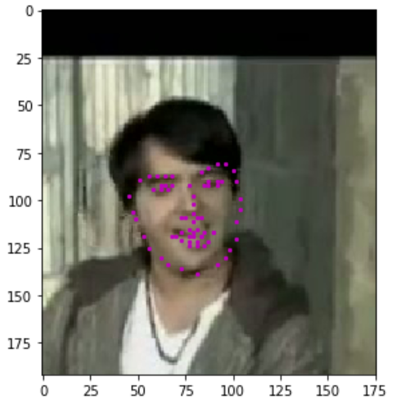
Facial Keypoints are also called Facial Landmarks which generally specify the areas of the nose, eyes, mouth, etc on the face, classified by 68 key points, with coordinates (x, y), for that face. With Facial Keypoints, we can achieve facial recognition, emotion recognition, etc.

Selecting the Dataset:

We’ll be using YouTube Faces Dataset. It is a dataset that contains 3,425 face videos designed for studying the problem of unconstrained face recognition in videos. These videos have been fed through processing steps and turned into sets of image frames containing one face and the associated keypoints.

Training and Test Data:

This facial keypoints dataset consists of 5770 color images. All of these images are separated into either a training or a test set of data. 3462 of these images are training images, for you to use as you create a model to predict keypoints. 2308 are test images, which will be used to test the accuracy of your model.

Pre-Processing the Data:

In order to feed the data(images) into the neural network, we have to transform the images into a fixed dimensional size and a standard color range by converting the numpy arrays to Pytorch Tensorsfor faster computation.

Transforms:

Normalize:

to convert a color image to grayscale values with a range of [0, 1] and normalize the keypoints to be in a range of about [-1, 1].
Rescale:

to rescale an image to a desired size.
RandomCrop:

to crop an image randomly.
ToTensor:

to convert numpy images to torch images.

Using Transformation techniques:

# test out some of these transforms
rescale = Rescale(100)
crop = RandomCrop(50)
composed = transforms.Compose([Rescale(250),
                               RandomCrop(224)])

# apply the transforms to a sample image
test_num = 500
sample = face_dataset[test_num]
fig = plt.figure()
for i, tx in enumerate([rescale, crop, composed]):
    transformed_sample = tx(sample)
    ax = plt.subplot(1, 3, i + 1)
    plt.tight_layout()
    ax.set_title(type(tx).__name__)
    show_keypoints(transformed_sample['image'], transformed_sample['keypoints'])
plt.show()

Output of Transformation:

Creating the Transformed Dataset:

# define the data tranform
# order matters! i.e. rescaling should come before a smaller crop
data_transform = transforms.Compose([Rescale(250),
                                     RandomCrop(224),
                                     Normalize(),
                                     ToTensor()])

# create the transformed dataset
transformed_dataset = FacialKeypointsDataset(csv_file='/data/training_frames_keypoints.csv',
                                             root_dir='/data/training/',
                                             transform=data_transform)

Here 224 * 224px are standardized input image size that is obtained by transforms and the output class scores shall be 136 i.e. 136/2 = 68

Define the CNN Architecture:

After you’ve looked at the data you’re working with and, in this case, know the shapes of the images and of the keypoints, you are ready to define a convolutional neural network that can learn from this data.

Define all the layers of this CNN, the only requirements are:

This network takes in a square (same width and height), grayscale image as input.
It ends with a linear layer that represents the keypoints (Last layer output 136 values, 2 for each of the 68 keypoint (x, y) pairs).

Shape of a Convolutional Layer:

K — out_channels : the number of filters in the convolutional layer

F — kernel_size

S — the stride of the convolution

P — the padding

W — the width/height (square) of the previous layer

The self.conv1 = nn.Conv2d(in_channels, out_channels, kernel_size, stride=1, padding=0)

output size = (W-F)/S +1 = (224–5)/1 +1 = 220, the output Tensor for one image will have the dimensions: (1, 220, 220)

1 = input image channel (grayscale), 32 = output channels/feature maps, 5x5 = square convolution kernel

CNN Architecture:

self.conv1 = nn.Conv2d(1, 32, 5)
# output size = (W-F)/S +1 = (224-5)/1 + 1 = 220
self.pool1 = nn.MaxPool2d(2, 2)
# 220/2 = 110  the output Tensor for one image, will have the dimensions: (32, 110, 110)

self.conv2 = nn.Conv2d(32,64,3)
# output size = (W-F)/S +1 = (110-3)/1 + 1 = 108
self.pool2 = nn.MaxPool2d(2, 2)
#108/2=54   the output Tensor for one image, will have the dimensions: (64, 54, 54)

self.conv3 = nn.Conv2d(64,128,3)
# output size = (W-F)/S +1 = (54-3)/1 + 1 = 52
self.pool3 = nn.MaxPool2d(2, 2)
#52/2=26    the output Tensor for one image, will have the dimensions: (128, 26, 26)

self.conv4 = nn.Conv2d(128,256,3)
# output size = (W-F)/S +1 = (26-3)/1 + 1 = 24
self.pool4 = nn.MaxPool2d(2, 2)
#24/2=12   the output Tensor for one image, will have the dimensions: (256, 12, 12)

self.conv5 = nn.Conv2d(256,512,1)
# output size = (W-F)/S +1 = (12-1)/1 + 1 = 12
self.pool5 = nn.MaxPool2d(2, 2)
#12/2=6    the output Tensor for one image, will have the dimensions: (512, 6, 6)

#Linear Layer
self.fc1 = nn.Linear(512*6*6, 1024)
self.fc2 = nn.Linear(1024, 136)

We can add Dropouts for Regularizing Deep Neural Networks. One of the secrets to achieving better results is to keep the probability(p) of dropouts within the range of 0.1 to 0.5. also, it’s better to have multiple dropouts of varying values of probability(p).

self.drop1 = nn.Dropout(p = 0.1)
self.drop2 = nn.Dropout(p = 0.2)
self.drop3 = nn.Dropout(p = 0.25)
self.drop4 = nn.Dropout(p = 0.25)
self.drop5 = nn.Dropout(p = 0.3)
self.drop6 = nn.Dropout(p = 0.4)

Next, We’ll construct our Feed-Forward Network having ReLU as our activation function.

Feedforward Neural Network:

    def forward(self, x):
        ## TODO: Define the feedforward behavior of this model
        ## x is the input image and, as an example, here you may choose to include a pool/conv step:
        ## x = self.pool(F.relu(self.conv1(x)))
      
        x = self.pool1(F.relu(self.conv1(x)))
        x = self.drop1(x)
        x = self.pool2(F.relu(self.conv2(x)))
        x = self.drop2(x)
        x = self.pool3(F.relu(self.conv3(x)))
        x = self.drop3(x)
        x = self.pool4(F.relu(self.conv4(x)))
        x = self.drop4(x)
        x = self.pool5(F.relu(self.conv5(x)))
        x = self.drop5(x)
        x = x.view(x.size(0), -1)
        x = F.relu(self.fc1(x))
        x = self.drop6(x)
        x = self.fc2(x)
        # a modified x, having gone through all the layers of your model, should be returned
        return x

Create the transformed Facial Keypoints Dataset, just as before

# create the transformed dataset
transformed_dataset = FacialKeypointsDataset(csv_file='/data/training_frames_keypoints.csv',
                                             root_dir='/data/training/',
                                             transform=data_transform)


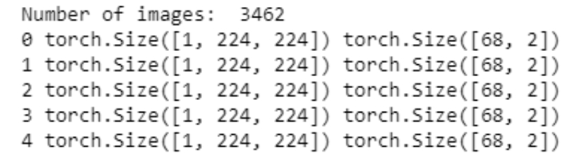
print('Number of images: ', len(transformed_dataset))

# iterate through the transformed dataset and print some stats about the first few samples
for i in range(4):
    sample = transformed_dataset[i]
    print(i, sample['image'].size(), sample['keypoints'].size())

Batching and loading data
Next, having defined the transformed dataset, we can use PyTorch’s DataLoader class to load the training data in batches of whatever size as well as to shuffle the data for training the model.

# load training data in batches
batch_size = 10

train_loader = DataLoader(transformed_dataset, 
                          batch_size=batch_size,
                          shuffle=True, 
                          num_workers=0)

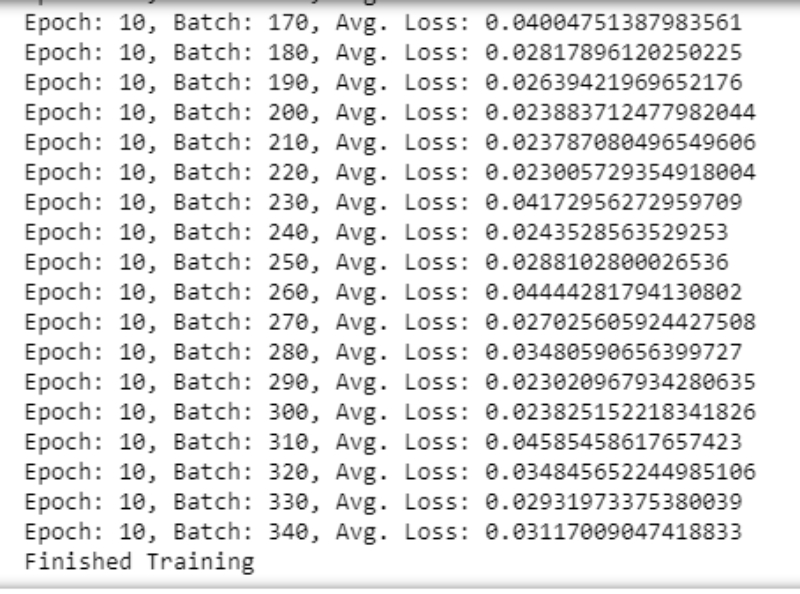
Train the CNN Model and Track the loss

## TODO: Define the loss and optimization
import torch.optim as optim

criterion = nn.SmoothL1Loss()

optimizer = optim.Adam(net.parameters(), lr = 0.001)

Note: Please try using a different criterion Loss function and also have the value of the learning rate set to the lowest number possible; in this case(0.001).

Training and Initial Observation
To quickly observe how our model is training and decide on whether or not we should modify its structure or hyperparameters, you’re encouraged to start off with just one or two epochs at first. As you train, note how your model’s loss behaves over time: does it decrease quickly at first and then slow down? Does it take a while to decrease in the first place? What happens if we change the batch size of your training data or modify your loss function? etc.
Use these initial observations to make changes to your model and decide on the best architecture before you train for many epochs and create a final model.
Training Loss:

Once you’ve found a good model, save it. So that you can load and use it later.
After you’ve trained a neural network to detect facial keypoints, you can then apply this network to any image that includes faces.
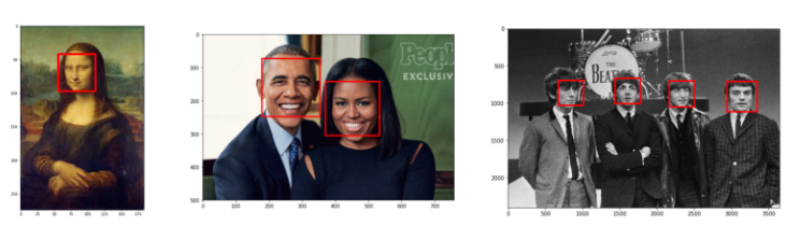
Detect faces in any image using Haar Cascade Detector in the project

# load in a haar cascade classifier for detecting frontal faces
face_cascade = cv2.CascadeClassifier('detector_architectures/haarcascade_frontalface_default.xml')

# run the detector
# the output here is an array of detections; the corners of each detection box
# if necessary, modify these parameters until you successfully identify every face in a given image
faces = face_cascade.detectMultiScale(image, 1.2, 2)

# make a copy of the original image to plot detections on
image_with_detections = image.copy()

# loop over the detected faces, mark the image where each face is found
for (x,y,w,h) in faces:
    # draw a rectangle around each detected face
    # you may also need to change the width of the rectangle drawn depending on image resolution
    cv2.rectangle(image_with_detections,(x,y),(x+w,y+h),(255,0,0),3) 

fig = plt.figure(figsize=(9,9))

plt.imshow(image_with_detections)

Haar Cascade Detector

Transform each detected face into an input Tensor

You’ll need to perform the following steps for each detected face:
1. Convert the face from RGB to grayscale
2. Normalize the grayscale image so that its color range falls in [0,1] instead of [0,255]
3. Rescale the detected face to be the expected square size for your CNN (224x224, suggested)
4. Reshape the numpy image into a torch image

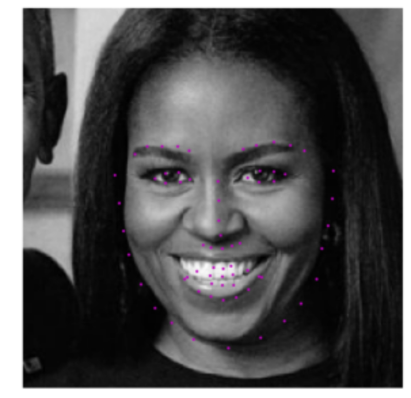
Detect and display the predicted keypoints

After each face has been appropriately converted into an input Tensor for our network to see as input, we can apply the network to each face. The output should be the predicted facial keypoints.
These keypoints will need to be “un-normalized” for display, and you may find it helpful to write a helper function like show_keypoints.

def showpoints(image,keypoints):
    
    plt.figure()
    
    keypoints = keypoints.data.numpy()
    keypoints = keypoints * 60.0 + 68
    keypoints = np.reshape(keypoints, (68, -1))
    
    plt.imshow(image, cmap='gray')
    plt.scatter(keypoints[:, 0], keypoints[:, 1], s=50, marker='.', c='r')
    

from torch.autograd import Variable
image_copy = np.copy(image)

# loop over the detected faces from your haar cascade
for (x,y,w,h) in faces:
    
    # Select the region of interest that is the face in the image 
    roi = image_copy[y:y+h,x:x+w]

    ## TODO: Convert the face region from RGB to grayscale
    roi = cv2.cvtColor(roi, cv2.COLOR_RGB2GRAY)
    image = roi

    ## TODO: Normalize the grayscale image so that its color range falls in [0,1] instead of [0,255]
    roi = roi/255.0
    
    ## TODO: Rescale the detected face to be the expected square size for your CNN (224x224, suggested)
    roi = cv2.resize(roi, (224,224))
    
    ## TODO: Reshape the numpy image shape (H x W x C) into a torch image shape (C x H x W)
    roi = np.expand_dims(roi, 0)
    roi = np.expand_dims(roi, 0)
    
    ## TODO: Make facial keypoint predictions using your loaded, trained network 
    roi_torch = Variable(torch.from_numpy(roi))
    
    roi_torch = roi_torch.type(torch.FloatTensor)
    keypoints = net(roi_torch)

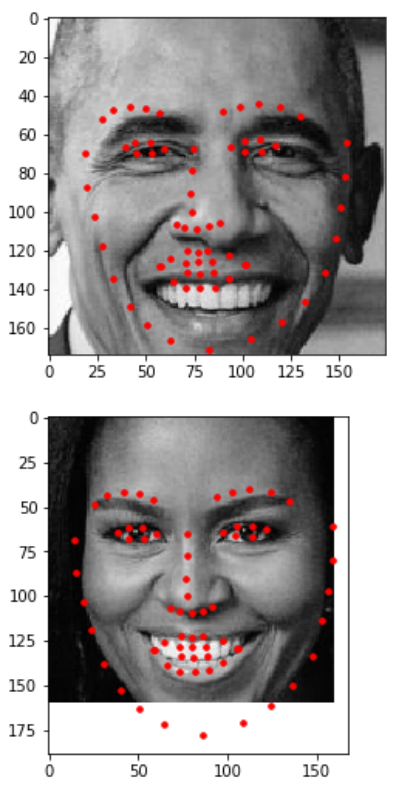
    ## TODO: Display each detected face and the corresponding keypoints        
    showpoints(image,keypoints)

Output:

Feel free to check out my project on Github.

Facial Keypoint Detection using CNN & PyTorch

Published by Krunal Kshirsagar

Selecting the Dataset:

Training and Test Data:

Pre-Processing the Data:

Transforms:

`Normalize`:

`Rescale`:

`RandomCrop`:

`ToTensor`:

Define the CNN Architecture:

Define all the layers of this CNN, the only requirements are:

CNN Architecture:

Feedforward Neural Network:

Transform each detected face into an input Tensor

Detect and display the predicted keypoints

Output:

Facial Keypoint Detection using CNN & PyTorch

Published by Krunal Kshirsagar

Selecting the Dataset:

Training and Test Data:

Pre-Processing the Data:

Transforms:

Normalize:

Rescale:

RandomCrop:

ToTensor:

Define the CNN Architecture:

Define all the layers of this CNN, the only requirements are:

CNN Architecture:

Feedforward Neural Network:

Transform each detected face into an input Tensor

Detect and display the predicted keypoints

Output:

`Normalize`:

`Rescale`:

`RandomCrop`:

`ToTensor`: